The Three Approaches To Value: Sales Comparison, Cost, and Income Capitalization

In a nutshell:

Real estate is valued by an appraiser who considers one or more of the three approaches to value:

• The Sales Comparison Approach evaluates sales of properties that are similar to a subject property.  After differences are accounted for, the comparables should represent a reasonable value range for the subject.
• The Cost Approach calculates the cost to construct new improvements on a site, less any depreciation due to age or other factors.  This depreciated cost is then added to the value of the underlying land.
• The Income Capitalization Approach measures the present worth of (a) future income generated by a property and (b) its eventual resale value.

In depth:

In appraisals of real estate, appraisers are most frequently asked to develop an independent and unbiased opinion of market value for a subject property.

Market value is determined by an appraiser who analyzes three types of market data: comparable sales, cost to replace (or reproduce), and income.  The process of analyzing data from these sources is commonly referred to as “The Three Approaches To Value”.

The following discussion explains each approach.

Sales Comparison

“Sales Comparison is King” – Numerous Appraisal Institute Instructors

Sales Comparison is the approach to value that the public is probably most familiar with.  In this approach, real estate appraisers research and analyze sales of similar properties (“comparables” or “comps”) in order to compare them to a subject property.  Sales comparison is usually the most insightful valuation method when numerous timely sales of similar properties are available to study.

To the greatest extent possible, appraisers strive to find comparables that buyers would consider to be acceptable substitutes for the subject property.  When I select comps, I always ask myself the question: “If the subject property was not on the market, what would the most probable buyer purchase instead?”  The goal is to find the most timely sales of properties that an appraiser feels would compete with the subject property in the open market.

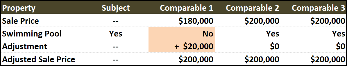
After comparables are selected, an appraiser develops his or her opinion of value by considering factors that buyers and sellers consider to be important.  In the case of a single family home, bedrooms, bathrooms, land area, ocean views, and age/quality of construction are among the factors that would typically be considered.  In most cases, mathematical adjustments are made to each comparable sale in order to allow for fair comparisons.  If a comparable has a superior trait, such as an extra bedroom, it is adjusted downward to match the subject.  If a comparable has an inferior trait, like a one car garage (instead of two at the subject), it may be adjusted upward to equate it to the subject property.

A Simple Adjustment Schedule

After all adjustments, the comparables should indicate the relevant range of values for the subject property.  The appraiser’s job is then to evaluate the strengths and weaknesses of the comparables and adjustments, and come to a value conclusion via the sales comparison approach.

Cost Approach 

Generally speaking, the cost approach is based on the idea that a rational real estate buyer would not usually pay meaningfully more for a property than it would cost to build new.  The cost approach is most useful in valuing new improvements.  In addition, it is often the best (and sometimes the only) method for valuing properties that are rarely sold and/or generate little or no income (such as schools, churches, parks,or military properties).

The cost approach involves three basic steps:

1. Estimating the cost to reproduce (or replace) the existing improvements .
2. Deducting any depreciation that is present.  (The most common form of depreciation is physical deterioration from age, but changing market tastes and external considerations can reveal types of depreciation known as “functional obsolescence” and “external obsolescence“, both of which I can discuss in a later article.)
3. Adding the value of the depreciated improvements to the value of the land underneath the property.  (The land is valued separately using the sales comparison approach.)

After land value is added to the depreciated value of improvements, the total represents the value of the property via the cost approach.

A side note for a future discussion:  It is common for appraisers to express the idea that the value indicated by the cost approach “sets the upper limit of value”.  Those interested in an in depth refutation of this concept are encouraged to obtain a copy of Nelson Bowes’ new book In Defense of the Cost Approach, published by the Appraisal Institute.

Income Capitalization Approach

The income approach is often summarized as “the present value of future benefits“.  Properties that generate positive cash flow can be appraised using a  “present value” or “time value of money” concept.  The income approach estimates the present value of (a) future income generated by a property and (b) its eventual resale value.

The term “capitalization” refers to the mechanism by which future income can be converted into a present value.  There are two types of capitalization: Direct and Yield.

Direct Capitalization considers one year of income and converts it to a property value.  The direct capitalization technique is often referred to as “Direct Cap” or using a “Cap Rate“.

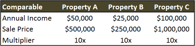
In my view, the simplest way to understand direct capitalization is using an “income multiplier“.  Consider the following chart:

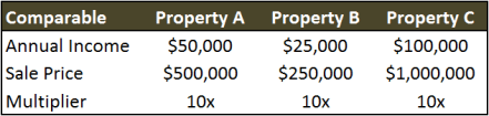
The three sales generate annual income of $50,000, $25,000 and $100,000 and sold for $500,000, $250,000, and $1,000,000, respectively.  In other words, each of the properties sold for 10 times their annual income.  Using this market data, it would be reasonable to conclude that the market is paying 10 times annual income for properties of this type.  Given this math, a property with annual income of say $75,000 would be valued at $750,000.

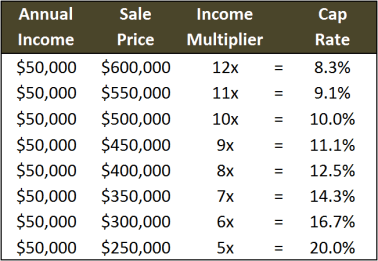
A “Cap Rate” is the inverse of an income multiplier.  If an income multiplier is 10x, which is the same thing as 10/1 (10 divided by 1), then the cap rate is 10% (1 divided by 10).

A 10x multiplier and 10% cap rate are too convenient.  Take a look at this chart to see how the relationship between multiplier and cap rate varies:

Yield Capitalization differs from Direct Capitalization in one fundamental way:  It considers multiple years of stabilized income and the eventual resale of the property.  The multiple years of income are converted to a present value using a “discount rate”.  The application of this process is sometimes called a “Discounted Cash Flow” or “DCF“.  Yield Capitalization considers multiple variables and can become very complex.  It is most appropriate for properties that are forecast to have uneven future cash flows (perhaps a large tenant is moving out in 3 years).  I’ll write more about this intricate valuation tool in a future article.

Comments and/or Questions?  Please leave them in the comments section below–I’d be happy to clarify or expand.

Aloha, Chris